A Data Scientist's Guide to the S&P 500

Stefan Obradovic
Published Online: December 21st, 2020, University of Maryland, College Park
Introduction
In 2008, Warren Buffett, a multi-billion dollar career investor and CEO of Berkshire Hathaway[1], made a \$1 million bet with the Hedge Fund Industry. His bet was that, accounting for fees, the S&P500 index would outperform a professionally curated Hedge Fund stock portfolio over 10 years. Protégé Partners LLC, an asset management firm based in Manhattan, New York took up the bet and 10 years later named Buffett the winner. In fact, Buffett claimed a staggering win. During the 10-year period the S&P500 gained an average of 7.1% per year, compared to 2.2% per year for Protégé [2].
So what is the S&P500?
The S&P 500 is a stock market index that measures the performance of roughly 500 large American companies [3]. As of the date of publication, there is currently over $11.2 Trillion (USD) invested in the S&P500, representing about 80% of the US stock market's value [4]. As such, the performance of the S&P500 index has been used widely as a metric to roughly estimate the overall performance of the market[5]. In fact, the S&P500 and other similar index funds have been widely regarded by investment moguls, like Warren Buffett himself, as some of the easiest, safest, and most consistent investments[6]. Simply put this is because index funds, like the S&P500, have a couple of very desireable qualities:
1) It is incredibly easy to invest in the S&P500.
The easiest way to invest in the S&P 500 is to buy an exchange-traded fund (ETF) that replicates the performance of the S&P 500 by holding the same stocks and in the same proportions. Exchange-traded funds, or ETFs, are a type of investment fund traded on public stock exchanges like the New York Stock Exchange. The amount that you invest in an ETF is divided between all of the ETF's investments and as a shareholder of the ETF, you are entitled to share the profits[7]. Examples of ETFs that mimic the holdings of the S&P500 index include but are not limited to the SPDR S&P 500 ETF Trust (SPY), the iShares S&P 500 Growth ETF (IVW), the iShares Core S&P 500 ETF (IVV), the Vanguard 500 Index Fund ETF (VOO), the SPDR Portfolio S&P 500 ETF (SPLG), and the Schwab US Large-Cap ETF (SCHX). Shares for each of these ETFs can be purchased on any electronic trading platform like Robinhood or stockbroker like Fidelity, TDAmeritrade, Charles Schwab, and many others.
2) The S&P500 is very diverse.
In the stock market as a whole, stocks and industries will not always perform well. However, if you invest in different "types" of stocks, it is very unlikely that all of them will perform poorly at the same time. By diversifying your portfolio between stocks in multiple sectors, market capitalizations, countries of origin, etc., you can avoid severe declines in the value of your investments. This is because companies in the stock market are highly dependent on each other, or respond the same way to the same economic forces for many reasons[8]. For instance, if the Toyota car manufacturer were to announce a sudden recall of over 2 million vehicles, this would likely drive the demand up for Ford vehicles, increasing their stock price. While a health care company might remain unaffected, this sort of announcement would often ripple throughout the market. American Airlines might see an increase in their stock price as more people opt for air travel and the raw materials manufacturer Steel Dynamics might see an increase in their stock price as well as Toyota looks to buy excess steel. Overall, the S&P500 is composed of over 500 companies in Communication Services, Consumer Discretionary, Consumer Staples, Energy, Financials, Health Care, Industrials, Information Technology, Materials, Real Estate, and Utilities[9]. As such, it has the quality of broad diversification which is extremely desireable for portfolio managers.
3) In the long-term, the S&P500 has large, positive returns.
At the end of the day, what really matters for investment portfolios is positive returns. No one would like to lose money on their investment. Since its inception in 1926, the S&P500 has grown approximately 9.8% each year. Additionally, the S&P500 increased annually 70% of the time, and saw losses only 30% of the time[10]. What this means is that for long-term investors, the S&P500 almost guarantees positive returns.
In summary, the goal of an investment portfolio is to spread the investment across a number of assets to minimize risk. Through diversification, we can pick a range of assets that minimize risk while maximizing potential returns.
So can we beat the S&P500?
Project Motivation
1) If we can better understand the composition of the S&P500, how each of these companies interact with each other, and what factors affect their stock prices, we can gain a deeper understanding of the benefits and pitfalls of the index.
2) We can potentially make a "better" S&P500 by subsetting only those stocks in the index that are the highest performers and minimally correlated with each other to further improve returns while retaining adequate portfolio diversification.
3) If we can predict future stock prices based on historical stock prices, we can buy stocks that we predict will perform well rather than holding all of the stocks in the S&P500.
Getting Started:
The following are required imports and prerequisite packages for the project:
import pandas as pd
import numpy as np
import datetime
import matplotlib.pyplot as plt
plt.rcParams['figure.figsize'] = (15, 9)
%matplotlib inline
import seaborn as sbn
import os
os.environ['KMP_DUPLICATE_LIB_OK']='True'
#Misc.
import psycopg2
from typing import Union, Tuple, List, Dict, Any, Optional
from pmdarima.arima import ADFTest
from sklearn.metrics import mean_squared_error
from fastdtw import fastdtw
import pmdarima as pm
from statsmodels.tsa.arima_model import ARIMA
import statsmodels.api as sm
import dtw
#Scipy - Clustering and Statistics
import scipy
import scipy.cluster.hierarchy as sch
from scipy import stats
from scipy.cluster.hierarchy import dendrogram, linkage
from scipy.spatial.distance import pdist, squareform, euclidean
#NetworkX - Graphs
import networkx as nx
import networkx
#RESTful APIs and Scraping
import requests
from urllib.request import urlopen, Request
from bs4 import BeautifulSoup
import bs4 as bs
# NLTK VADER for sentiment analysis
from nltk.sentiment.vader import SentimentIntensityAnalyzer
import nltk
import warnings
warnings.filterwarnings("ignore")
Resources for going deeper into these packages:
Part 1: Data Collection and Processing
First, we scrape Wikipedia to get a list of companies in the S&P500, their corresponding tickers on the New York Stock Exchange, and the Sector that the company falls under based on the Global Industry Classification Standard (GICS).
#Send a GET request to the Wikipedia API
resp = requests.get('http://en.wikipedia.org/wiki/List_of_S%26P_500_companies') #Returns the html of the Wikipedia page for S&P500 companies
soup = bs.BeautifulSoup(resp.text, 'lxml') #Parse the webpage from Wikipedia with BeautifulSoup
table = soup.find('table', {'class': 'wikitable sortable'}) #Find the contents under the table tag
tickers = [] #Stores tickers
names = [] #Stores company names
industries = [] #Stores GICS Industry
for row in table.findAll('tr')[1:]: #Iterates through each row in the table excluding the header and extracts relevant data
tickers.append(row.findAll('td')[0].text)
names.append(row.findAll('td')[1].text)
industries.append(row.findAll('td')[3].text)
tickers = [s.replace('\n', '') for s in tickers] #delete newline characters in parsed data
stock_info = pd.DataFrame({'Ticker': tickers, 'Name': names, 'Sector': industries}) #Create Dataframe from Wikipedia data
stock_info = stock_info.replace('Communication Services\n','Communication Services') #Clean messy data
stock_info = stock_info.sort_values(by=['Ticker'], ignore_index = True) #Sort Alphabetically by Ticker
stock_info.head()
print(f' Number of stocks in stock_info: {stock_info.shape[0]}')
We set the time-window for this analysis to be between April 1st of 2019 and December 1st of 2019
start_date = datetime.datetime(2019, 4, 1)
end_date = datetime.datetime(2019, 12, 1)
Next, we will establish a connection to a PostgreSQL Database.
The database we will be using to query data is owned by the Smith Investment Fund, a student investment group at the University of Maryland (linked here). This database houses both equity and fundamental data purchased from Quandl, a premier source for financial and investment data.
The Quandl Fundamental Data (linked here) is updated daily and provides up to 20 years of history for 150 essential fundamental indicators and financial ratios, for more than 14,000 US public companies. Fundamental indicators are publically reported ratios and values related to economic and financial factors of a company including the balance sheet, statement of cash flows, the income statement, and Statement of Stockholder's Equity along with any strategic initiatives, microeconomic indicators, and consumer behavior recorded by the company.
The Quandl Equity Data (linked here) is updated daily and offers end of day prices, dividends, adjustments, and stock splits for US publicly traded stocks since 1996.
Code for this has section has been ommitted for privacy reasons
From the database, extract the following Fundamental Factors for each stock in the S&P500:
Earnings Before Interest, Taxes, Depreciation, and Amortization ('ebitda'): This indicator measures the overall financial performance, or profitability, of a company. It is oftentimes more accurate an indicator because it represents earnings before accounting and financial deductions.
$EBITDA = NET INCOME + INTEREST + TAXES + DEPRECIATION + AMORTIZATION$
Earnings per Share ('eps'): This indicator measures how much money a company makes for each share of its stock, an indication of corporate value. The larger the Earnings per Share, the more profitable the company is.
$Earnings per Share = \frac{Net Income - Preferred Dividends}{End-of-Period Common Shares Outstanding}$
Enterprise Value ('ev'): This indicator measures the enterprise value of a company, including market capitalization adjusted for short-term and long-term debts as well as any cash on the balance sheet. This is often viewed as the "selling price" that a company would go for.
$Enterprise Value = Market Capitalization + Total Debt - Cash$
Gross Profit Margin ('grossmargin') This indicator measures the portion of each dollar of revenue that a company retains as gross profit.
$Gross Profit = Sales - Cost of Goods Sold$
Price to Earnings Ratio ('pe'): This indicator shows the current share price relative to the Earnings Per Share of a company. Investors use this ratio to determine the relative value of a company's shares.
$P/E = \frac{Market Value per Share}{Earnings per Share}$
Research and Development ('rnd'): This indicator measures a company's activities in driving innovation and development of products to produce new products or services.
Also extract Equity Data for each company in the S&P500
Opening Price ('open'): The opening price for a stock is the price exactly at the opening of trading in the New York Stock Exchange at 9:30am EST.
High Price ('high'): The high price for a stock is the peak intraday price of a stock.
Low Price ('low'): The low price for a stock is the lowest intraday price of a stock.
Adjusted Closing Price ('close'): The adjusted closing price is the closing price of a stock adjusted for stock splits, dividends, and rights offerings.
Volume ('volume'): The amount of stocks that change hands over the course of a day for a given company.
Dividends ('dividends'): The distribution a portion of a company's earnings to preferred stockholders.
Unadjusted Closing price ('closeunadj'): The close price for a stock is the price exactly at the close of the New York Stock Exchange at 4:00pm EST.
In this project, we will be using exclusively the Adjusted Closing price
def extract_data(stocks, start_date, end_date):
"""Queries the PostgreSQL database for Equity and Financial data
for the given list of stocks between the start date and the end date
Args:
stocks: A list of tickers
start_date: A datetime object representing the start date
end_date: A datetime object representing the end date
Returns:
Two dataframes, the first one being equity data and the second
being the fundamental data
"""
fundamental = get_fundamental_filled(stocks, start_date, end_date,
['ebitda',
'eps',
'ev',
'grossmargin',
'pe',
'rnd',
'marketcap'])
equity_data = get_equity_data(stocks, start_date, end_date)
return equity_data, fundamental
We separate the time series data for each variable for each stock into separate dataframes for each variable of interest
#Extract Equity Data and Fundamental Data for each ticker in the S&P500
equity_data, fundamental_data = extract_data(tickers, start_date, end_date)
#Create Dataframes for each variable of interest where columns correspond to the ticker and rows correspond to the date
#EQUITY
close_data = equity_data['close']
#FUNDAMENTAL
ebitda_data = fundamental_data['ebitda']
eps_data = fundamental_data['eps']
ev_data = fundamental_data['ev']
gm_data = fundamental_data['grossmargin']
pe_data = fundamental_data['pe']
rnd_data = fundamental_data['rnd']
mc_data = fundamental_data['marketcap']
ebitda_data.index.names = ['date']
eps_data.index.names = ['date']
ev_data.index.names = ['date']
gm_data.index.names = ['date']
pe_data.index.names = ['date']
rnd_data.index.names = ['date']
mc_data.index.names = ['date']
Unfortunately, we don't have fundamental data available for every stock in the S&P500
print(f' Number of stocks in close_data: {close_data.shape[1]}')
print(f' Number of stocks in ev_data: {ev_data.shape[1]}')
print(f' Number of stocks in stock_info: {stock_info.shape[0]}')
To account for this, we prune the equity data to the size of the available fundamental data
# For the list of tickers in the S&P500, drop tickers that aren't present in the fundamental data
for ind, x in stock_info['Ticker'].items():
if x not in ev_data.columns:
stock_info = stock_info[stock_info.Ticker != x]
#For each ticker in the close price dataframe, drop tickers that aren't represent in the fundamental data
for x in close_data.columns:
if x not in ev_data.columns:
close_data.drop([x], axis=1, inplace=True)
stock_info.reset_index(inplace = True, drop = True)
print(f' Number of stocks in close_data: {close_data.shape[1]}')
print(f' Number of stocks in ev_data: {ev_data.shape[1]}')
print(f' Number of stocks in stock_info: {stock_info.shape[0]}')
Next, we check for the presence of missing data in the datasets
print(f'NaN data in stock_info: {stock_info.isna().sum().sum()}')
print(f'NaN data in close_data: {close_data.isna().sum().sum()}')
print(f'NaN data in ebitda_data: {ebitda_data.isna().sum().sum()}')
print(f'NaN data in gm_data: {gm_data.isna().sum().sum()}')
print(f'NaN data in pe_data: {pe_data.isna().sum().sum()}')
print(f'NaN data in eps_data: {eps_data.isna().sum().sum()}')
print(f'NaN data in ev_data: {ev_data.isna().sum().sum()}')
print(f'NaN data in rnd_data: {rnd_data.isna().sum().sum()}')
print(f'NaN data in mc_data: {mc_data.isna().sum().sum()}')
Since there are missing data, we forward fill NaN values, then backward fill for entries that start with NaNs. Dropping rows that include NaNs would greatly diminish the size of the datasets and lead to information loss. We start by forward filling the data because fundamental factors remain relatively constant on a day-to-day time-scale. This is because fundamental factors are often reported by companies on a quarterly basis, or 4 times per year$^{[11]}$.
close_data.fillna(method='ffill', inplace=True)
close_data.fillna(method='bfill', inplace=True)
ebitda_data.fillna(method='ffill', inplace=True)
ebitda_data.fillna(method='bfill', inplace=True)
eps_data.fillna(method='ffill', inplace=True)
eps_data.fillna(method='bfill', inplace=True)
ev_data.fillna(method='ffill', inplace=True)
ev_data.fillna(method='bfill', inplace=True)
gm_data.fillna(method='ffill', inplace=True)
gm_data.fillna(method='bfill', inplace=True)
pe_data.fillna(method='ffill', inplace=True)
pe_data.fillna(method='bfill', inplace=True)
pe_data.dropna(axis=1, inplace=True)
rnd_data.fillna(method='ffill', inplace=True)
rnd_data.fillna(method='bfill', inplace=True)
mc_data.fillna(method='ffill', inplace=True)
mc_data.fillna(method='bfill', inplace=True)
print(f'NaN data in stock_info: {stock_info.isna().sum().sum()}')
print(f'NaN data in close_data: {close_data.isna().sum().sum()}')
print(f'NaN data in ebitda_data: {ebitda_data.isna().sum().sum()}')
print(f'NaN data in gm_data: {gm_data.isna().sum().sum()}')
print(f'NaN data in pe_data: {pe_data.isna().sum().sum()}')
print(f'NaN data in eps_data: {eps_data.isna().sum().sum()}')
print(f'NaN data in ev_data: {ev_data.isna().sum().sum()}')
print(f'NaN data in rnd_data: {rnd_data.isna().sum().sum()}')
print(f'NaN data in mc_data: {mc_data.isna().sum().sum()}')
When we check the closing price data, we can see that we still have data missing for some days. This is because stock exchanges, like the New York Stock Exchange, follow a regular work week, where markets are closed on weekends and holidays$^{[12]}$. This makes our time-series data non-continous.
close_data.head(10)
To account for this missing aspect of the data, we further forward fill the data for missing dates. This is the most logical thing to do since stocks are not traded, the actual price of the stock remains unchanged (even though perceptions of the stock's price continue to change). We expect that on Monday market open, after the weekend break, that stock prices change more drastically on average from their Friday closing price than close/open prices do throughout the work week.
close_data = close_data.resample('D').ffill().reset_index()
close_data.set_index('date', inplace=True)
ebitda_data = ebitda_data.resample('D').ffill()
eps_data = eps_data.resample('D').ffill()
ev_data = ev_data.resample('D').ffill()
gm_data = gm_data.resample('D').ffill()
pe_data = pe_data.resample('D').ffill()
rnd_data = rnd_data.resample('D').ffill()
mc_data = mc_data.resample('D').ffill()
close_data.head(10)
Next, we query the database for the closing price of the S&P500 Index as a whole
# Get the S&P500 closing price
sp_data = get_sp_close(start_date, end_date)
sp_data = sp_data.resample('D').ffill().reset_index()
sp_data.set_index('date', inplace=True)
So how well has the S&P500 performed in this time period?
fig, ax = plt.subplots(figsize=(10,10))
ax.plot(sp_data.index, sp_data, label = 'Daily SPY')
ax.plot(sp_data.rolling(10).mean(), label = '10 Day Rolling Mean')
ax.plot(sp_data.rolling(30).mean(), label = '30 Day Rolling Mean')
ax.plot(sp_data.rolling(100).mean(), label = '100 Day Rolling Mean')
ax.set_title('S&P500 Closing Price')
ax.set_xlabel('Date')
ax.set_ylabel('Closing price (in USD)')
ax.legend()
fig.show()

print('S&P500 returns between April 1, 2019 and December 1, 2019: ' + str((sp_data['close'][-1]-sp_data['close'][0])/sp_data['close'][0]*100)+ '%')
Throughout the year, for most days, the S&P500 had close to 0% daily returns. The 11% returns calculated above are largely due to one month (November to December) of high average returns near the end of the period
fig, ax = plt.subplots(figsize=(8,8))
ax.plot(sp_data.index, stats.zscore(sp_data), label = 'SPY')
ax.set_title("Z-scored Clsoing Price for S&P500")
ax.set_ylabel("Standard Deviations away from mean closing price")
ax.set_xlabel("Date")
plt.show()

From the above figure, the S&P500 had closing prices ~1 to 2 standard deviations below the mean at the beginning of the year and ~1 to 2 standard deviations above the mean at the end of the period
sp_data.pct_change().plot.hist(bins = 60)
plt.xlabel("Daily returns %")
plt.ylabel("Frequency")
plt.title("S&P500 daily returns data")
plt.text(-0.03,100,"Extremely Low\nreturns")
plt.text(0.02,100,"Extremely High\nreturns")
plt.show()

The histogram above shows that most days saw litte to no returns and that the S&P500 had more good days than bad days between April and December of 2019
Which stocks in the S&P500 have the highest EBITDA?
top_20_ebitda = ebitda_data.mean().sort_values(ascending=False)[0:20]
fig, ax = plt.subplots(figsize=(20,8))
ax.bar(top_20_ebitda.index,top_20_ebitda.to_numpy())
ax.set_title('Companies with highest EBIDTA')
fig.show()

Berkshire Hathaway, Apple, Microsoft, AT&T, and Google have the highest EBIDTA. This indicates that these companies have the highest overall financial performance/profitability.
Which stocks in the S&P500 have the highest Earnings per Share?
top_20_eps = eps_data.mean().sort_values(ascending=False)[0:20]
fig, ax = plt.subplots(figsize=(15,8))
ax.bar(top_20_eps.index,top_20_eps.to_numpy())
ax.set_title('Companies with highest Earnings per Share')
fig.show()

NVR (A home construction company), Booking Holdings (owner of Kayak, Priceline, and Booking.com), Autozone, and Bio-Rad labratories have the highest Earnings per Share. This indicates that these companies are the most profitable (make the most money per share of stock).
Which companies in the S&P500 have the highest Price to Earnings Ratio?
top_20_pe = pe_data.mean().sort_values(ascending=False)[0:20]
fig, ax = plt.subplots(figsize=(15,8))
ax.bar(top_20_pe.index,top_20_pe.to_numpy())
ax.set_title('Companies with highest Price to Earnings Ratio')
fig.show()

Weyerhaeuser (Real Estate Investment Company), ServiceNow (Software Company), Cardinal Health, and Live Nation Entertainment have the highest Price to Earnings Ratio. These companies either have the highest potential for growth or are the most overvalued.
Which companies in the S&P 500 have the highest Research and Development?
top_20_rnd = rnd_data.mean().sort_values(ascending=False)[0:20]
fig, ax = plt.subplots(figsize=(20,8))
ax.bar(top_20_rnd.index,top_20_rnd.to_numpy())
ax.set_title('Companies with highest Research and Development Costs')
fig.show()

Amazon, Google, Microsoft, Apple, Intel, and Facebook are the companies with the highest spending towards research and development. All of these companies are in the technology sector. Following these companies are all of the largest Health Care companies like Johnson and Johnson, Merck, Abbvie, and Pfizer.
Which companies in the S&P have the highest Enterprise Value?
top_20_ev = ev_data.mean().sort_values(ascending=False)[0:20]
fig, ax = plt.subplots(figsize=(20,8))
ax.bar(top_20_ev.index,top_20_ev.to_numpy())
ax.set_title('Companies with highest Enterprise Value')
fig.show()

Apple, Amazon, Microsoft, Google, JPMorgan Chase, Berkshire Hathaway, and Facebook all have the largest Enterprise Value. These companies also happen to be in the top 10 companies in the S&P500 by market cap.
So What Sectors Make up the S&P500?
frequencies = stock_info.groupby('Sector').size()
fig1, ax1 = plt.subplots(figsize=(10,10))
ax1.pie(frequencies, labels=frequencies.index, autopct='%1.1f%%', startangle=90, )
ax1.axis('equal') # Equal aspect ratio ensures that pie is drawn as a circle.
plt.show()

From the above pie chart, we can see the top 2 largest sectors represented in the S&P500: 14.5% of companies in the S&P500 are Technology companies and 14.3% are Industrial companies
The two lowest represented sectors in the S&P500 are Communication Services at 4.4% and Energy at 5.1%
Overall, the S&P500 is heavily biased towards Technology, Financial Services, Industrials, and Health Care companies.
#Calculate the total market cap of the top 10 companies in the S&P500
top_10_mc = mc_data.iloc[-1,].sort_values(ascending=False)[0:10].sum()
#Calculate total market cap of the S&P500
all_mc = mc_data.iloc[-1,].sort_values(ascending=False).sum()
print("\nPercent of Total S&P500 Market Capitalization Represented by top 10 stocks:")
print(top_10_mc/all_mc * 100)
top_20_mc = mc_data.iloc[-1].sort_values(ascending=False)[0:20]
fig, ax = plt.subplots(figsize=(15,8))
ax.bar(top_20_mc.index,top_20_mc.to_numpy())
ax.set_title("S&P500 Stocks with Largest Market Capitalization")
ax.set_ylabel('Market Capitalization')
ax.set_xlabel('Tickers')
fig.show()

In fact, the top 10 largest companies in the S&P500, representing about 24% of the index by market capitalization are Apple Inc., Microsoft, Amazon.com, Google, Facebook, Berkshire Hathaway, JPMorgan Chase & Co. and Visa Inc, Johnson & Johnson, and Walmart. (5 Technology companies, 3 financial companies, 1 Health Care company, and 1 Consumer Staples).
Conclusion: So maybe the S&P500 isn't actually diverse enough?
What is the Average Market Capitalization by Sector in the S&P500?
average_mc = mc_data.mean().sort_values(ascending=False)
frequencies = stock_info.groupby('Sector').size()
mc_sectors = frequencies.copy()
for i, row in mc_sectors.items():
mc_sectors[i] = 0
for i, row in stock_info.iterrows():
for j, row2 in average_mc.items():
if(stock_info.iloc[i]['Ticker'] == j):
for k, row3 in mc_sectors.items():
if (k == stock_info.iloc[i]['Sector']):
mc_sectors[k] += row2
for i, val in mc_sectors.items():
mc_sectors[i] /= frequencies[i]
mc_sectors
fig1, ax1 = plt.subplots(figsize=(10,10))
ax1.pie(mc_sectors, labels=mc_sectors.index, autopct='%1.1f%%', startangle=90, )
ax1.axis('equal') # Equal aspect ratio ensures that pie is drawn as a circle.
plt.show()

Although a handfull of Technology, Healthcare, and Financial companies in the top of the S&P500 represent around 24% of the total market capitalization of the S&P500, we can see from this graph above that the rest of the companies in these sectors have considerably lower market capitalization, making these sectors represent comparatively less total market capitalization overall. Communication Services represent the most of the S&P500 with 22.2% of the S&P market cap being represented by these companies, however, none of these companies are particularly high in market capitalization, so we can conclude that these companies have consistent market capitalization. The next largest sectors by market capitalization are information Technology and Consumer Staples.
What is the Average Enterprise Value (EV) by Sector in the S&P500?
average_ev = ev_data.mean().sort_values(ascending=False)
frequencies = stock_info.groupby('Sector').size()
ev_sectors = frequencies.copy()
for i, row in ev_sectors.items():
ev_sectors[i] = 0
for i, row in stock_info.iterrows():
for j, row2 in average_ev.items():
if(stock_info.iloc[i]['Ticker'] == j):
for k, row3 in ev_sectors.items():
if (k == stock_info.iloc[i]['Sector']):
ev_sectors[k] += row2
for i, val in ev_sectors.items():
ev_sectors[i] /= frequencies[i]
fig1, ax1 = plt.subplots(figsize=(10,10))
ax1.pie(ev_sectors, labels=ev_sectors.index, autopct='%1.1f%%', startangle=90, )
ax1.axis('equal') # Equal aspect ratio ensures that pie is drawn as a circle.
plt.show()

The results for enterprise value are very similar to those results seen by Market Capitalization. This is because both values measure a company's "worth", the exception being that enterprise value accounts for debts. As such there are a few notable differences in sectors between market capitalization and enterprise value. Firstly, the Financial Sector gained over 1.7% by enterprise value when compared to market capitalization. This indicates that Financial companies tend to be undervalued by market cap because they have little debt. On the other hand, companies in Information Technology and Healthcare tend to be overvalued by market cap because of higher debts incurred.
What is the average EBITDA by Sector in the S&P500?
average_ebitda = ebitda_data.mean().sort_values(ascending=False)
frequencies = stock_info.groupby('Sector').size()
ebitda_sectors = frequencies.copy()
for i, row in ebitda_sectors.items():
ebitda_sectors[i] = 0
for i, row in stock_info.iterrows():
for j, row2 in average_ebitda.items():
if(stock_info.iloc[i]['Ticker'] == j):
for k, row3 in ebitda_sectors.items():
if (k == stock_info.iloc[i]['Sector']):
ebitda_sectors[k] += row2
for i, val in ebitda_sectors.items():
ebitda_sectors[i] /= frequencies[i]
ebitda_sectors
fig1, ax1 = plt.subplots(figsize=(10,10))
ax1.pie(ebitda_sectors, labels=ebitda_sectors.index, autopct='%1.1f%%', startangle=90, )
ax1.axis('equal') # Equal aspect ratio ensures that pie is drawn as a circle.
plt.show()

From this graph we can see that Energy, Financial, and Communications companies have much larger earnings before interest, taxes, debts, and ammortization, where communication companies represent a significantly larger portion of earnings in the S&P500.
What is the Average Price to Earnings Ratio in the S&P by Sector?
average_pe = pe_data.mean().sort_values(ascending=False)
frequencies = stock_info.groupby('Sector').size()
pe_sectors = frequencies.copy()
for i, row in pe_sectors.items():
pe_sectors[i] = 0
for i, row in stock_info.iterrows():
for j, row2 in average_pe.items():
if(stock_info.iloc[i]['Ticker'] == j):
for k, row3 in pe_sectors.items():
if (k == stock_info.iloc[i]['Sector']):
pe_sectors[k] += row2
for i, val in pe_sectors.items():
pe_sectors[i] /= frequencies[i]
pe_sectors
fig1, ax1 = plt.subplots(figsize=(10,10))
ax1.pie(pe_sectors, labels=pe_sectors.index, autopct='%1.1f%%', startangle=90, )
ax1.axis('equal') # Equal aspect ratio ensures that pie is drawn as a circle.
plt.show()

High price to earnings ratio often indicates companies that are either overvalued, or have the highest potential for growth. Real Estate companies represent 45.9% of the total price to earnings of the S&P500. Real Estate is likely prime for growth and reaching overvalued as the industry has been steadily recovering since the 2008 Housing Crisis$^{[13]}$. Information Technology also likely has high price to earnings ratio since it has seen the largest growth in recent years and it is expected to only grow more in the comming years.
What is the Average Earnings per Share in the S&P500 by Sector?
average_eps = eps_data.mean().sort_values(ascending=False)
frequencies = stock_info.groupby('Sector').size()
eps_sectors = frequencies.copy().astype('float')
for i, row in eps_sectors.items():
eps_sectors[i] = 0
for i, row in stock_info.iterrows():
for j, row2 in average_eps.items():
if(stock_info.iloc[i]['Ticker'] == j):
for k, row3 in eps_sectors.items():
if (k == stock_info.iloc[i]['Sector']):
eps_sectors[k] += row2
for i, val in eps_sectors.items():
eps_sectors[i] = float(eps_sectors[i]/frequencies[i])
fig1, ax1 = plt.subplots(figsize=(10,10))
ax1.pie(eps_sectors, labels=eps_sectors.index, autopct='%1.1f%%', startangle=90, )
ax1.axis('equal') # Equal aspect ratio ensures that pie is drawn as a circle.
plt.show()

Overall, Consumer Discretionary comapanies represent the highest percentage of Earnings per share followed by Financial companies, this is likely because companies in these sectors have the lowest number of stock splits on average, meaning that they don't often increase the supply of their stock.
What is the Average Research and Development Spending by Sector in the S&P500?
average_rnd = rnd_data.mean().sort_values(ascending=False)
frequencies = stock_info.groupby('Sector').size()
rnd_sectors = frequencies.copy()
for i, row in rnd_sectors.items():
rnd_sectors[i] = 0
for i, row in stock_info.iterrows():
for j, row2 in average_rnd.items():
if(stock_info.iloc[i]['Ticker'] == j):
for k, row3 in rnd_sectors.items():
if (k == stock_info.iloc[i]['Sector']):
rnd_sectors[k] += row2
for i, val in rnd_sectors.items():
rnd_sectors[i] /= frequencies[i]
rnd_sectors
fig1, ax1 = plt.subplots(figsize=(10,10))
ax1.pie(rnd_sectors, labels=rnd_sectors.index, autopct='%1.1f%%', startangle=90, )
ax1.axis('equal') # Equal aspect ratio ensures that pie is drawn as a circle.
plt.show()

Overall, the three sectors that spend the most on research and development are Communication Services, Information Technology, and Health Care. This makes sense because each of these sectors are highly dependent on innovation and research to produce new products. Consumer Staples and Financials spend remarkably little on Research and Development, likely since these services remain similar and do not need much development.
Do fundamental factors explain change in price?
Fit a Linear Model to predict Apple's stock price using fundamental factors
frame = { 'close': close_data['AAPL'][:-2],
'ebidta': ebitda_data['AAPL'],
'eps': eps_data['AAPL'],
'ev': ev_data['AAPL'],
'gm': gm_data['AAPL'],
'pe': pe_data['AAPL'],
'rnd': rnd_data['AAPL'],
'mc': mc_data['AAPL']
}
AAPL = pd.DataFrame(frame)
AAPL.head()
#Fit a linear regression model using OLS in statsmodels (SciKit-Learn does not display summary statistics like p-value)
est = sm.OLS(AAPL['close'], AAPL[['ebidta', 'eps', 'ev', 'gm', 'pe', 'rnd', 'mc']])
est2 = est.fit()
print(est2.summary()) #Print summary statistics
The variance in the fundamental factors explains 77.8% of the variance in the closing price of AAPL. All of the fundamental factors are significantly linearly associated with the closing price of Apple.
Section 2:
What causes stock prices to change?
In short, just like any other commodity, stock prices are determined by the supply and demand of a company's stock$^{[14]}$

In an efficient market, the demand of a company's stock is equal to the supply of the stock available. If a company exceeds expected performance for the fiscal term, then investors will demand more of the company's stock, and since the supply of the company's stock does not increase as quickly in response, the price of it's stock goes up.
There are thousands and millions of factors that affect the supply and demand for a company's stock. However, there are three major categories of such factors$^{[15]}$:
Fundamental Factors:
* Fundamental factors drive stock prices based on a company's earnings and profitability from producing and selling goods and services.
* In an efficient market, stock prices would be determined primarily by fundamentals: i.e. "How well is the company performing?"
Technical Factors
* Technical factors relate to a stock's price history in the market pertaining to chart patterns, momentum, and behavioral factors of traders and investors.
* Technical factors are the mix of external conditions that alter the supply of and demand for a company's stock. Examples include inflation and economic strength of peers.
Overall Investor Sentiment
* Market sentiment is often subjective, biased, and obstinate. If investors dwell on a single piece of news or are "caught up in the hype", the stock becomes artificially high or low based on the fundamentals.
Assumption: On a short time-scale where fundamental factors remain constant (unreported), stock prices are mostly influenced by their previous prices. Overall investor sentiment and short-term investor "reactions" to moving stock prices can lead to high volatility and inefficiency in the market. With the proper statistical tools, these inefficiencies can be exploited for profit.
Goal: If we can model the dependency of stock prices on their previous prices, we can use this to predict future movements in the market and invest accordingly.
Hypothesis: ARIMA is a good enough model to exploit inefficiencies in the market caused by investor sentiment and is a reasonable tool for predicting future stock performance.
What is ARIMA? (Autoregressive Integrated Moving Average)
ARIMA models aim to describe autocorrelations in time-series data
ARIMA is a three-part model:
Autoregression (AR) refers to a model that shows a changing variable that regresses on its own lagged, or prior, values.
Integrated (I) represents the differencing of raw observations to allow for the time series to become stationary, i.e., data values are replaced by the difference between the data values and the previous values.
Moving average (MA) incorporates the dependency between an observation and a residual error from a moving average model applied to lagged observations.
In Essence: $$ f(x_t) = \sum_{i=1}^{p} (\alpha_i * f(x_{t-i})) + \sum_{j=1}^{q} (\beta_i * \epsilon_{t-j}) + \epsilon_t $$
The value at time-step t is determined by a weighted sum of the past t-1 to t-p time-steps plus a weighted sum of the past t-1 to t-q residual errors plus an error coefficient.
A standard notation would be ARIMA(p,d,q)
p: the number of lag observations in the model; also known as the lag order.
d: the number of times that the raw observations are differenced; also known as the degree of differencing.
q: the size of the moving average window; also known as the order of the moving average.
ARIMA models can also account for seasonal time series data. Seasonal ARIMA models are denoted with ARIMA(p,d,q)(P,D,Q)[m]
m refers to the number of periods in each season.
P,D,Q refer to the autoregressive, differencing, and moving average terms for the seasonal part of the ARIMA model.
Note: to determine whether or not the time series should be differenced, an Augmented Dicky-Fuller Test is performed. The null hypothesis is that a unit root exists in the time series, or in other words, there is an underlying stochastic trend, or systematic, yet unpredictable pattern. The alternative hypothesis is that the time series exhibits Stationarity, an assumption of the ARIMA model.
Special Cases:
An ARIMA(0, 1, 0) represents a random walk/random.htm) -> $X_{t}=X_{t-1}+\epsilon _{t}$
An An ARIMA(0, 0, 0) represents a white noise model
An ARIMA(0, 1, 2) model is a Damped Holt's model
An ARIMA(0, 1, 1) model is a basic exponential smoothing model -> $s_{t}=\alpha*x_{t-1}+(1-\alpha)*s_{t-1}$
How are ARIMA models selected?
Estimate out-of-sample prediction error with Akaike Information Criterion (AIC)
AIC estimates the relative amount of information lost by a given model: the less information a model loses, the higher the quality of that model. AIC deals with the trade-off between the goodness of fit of the model (overfitting) and the simplicity of the model (underfitting). A good model is one that minimizes AIC.
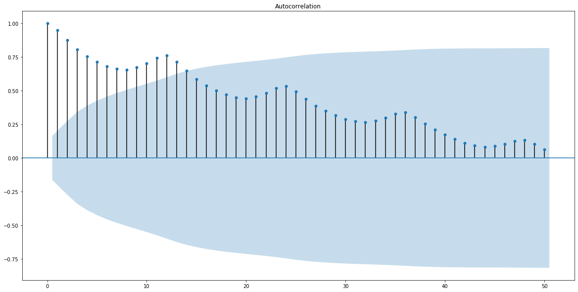
ACF Plot
ACF is an auto-correlation function calculates auto-correlation of a time series with its lagged values. Plotting these values along with the confidence interval describes how well the present value of the series is related with its past values. The number of lags that are outside of the confidence interval is the number of lags that are significantly autocorrelated.
PACF Plot
PACF is a partial auto-correlation function that calculates auto-correlation of the residuals. Plotting these values along with the confidence interval describes how well the present residual error of the time series is related with its past residual errors. The number of lags that are outside of the confidence interval is the number of residual error lags that are significantly autocorrelated.

While modeling, we don’t want to keep too many features which are correlated as that can create multicollinearity issues.
Use of ARIMA:
* In recent literature, ARIMA models are used as baseline performance measures to compare deep learning approaches like RNN LSTM.
* ARIMA predictions can also be used as engineered model parameters for Deep Learning models, and can be used in determining how "related" two Time-Series Objects are.
def predict_auto_arima(data, target, columns, split, days_ahead, verbose = True):
sbn.set(font_scale=1.2)
predicted_returns = {}
datasets = []
count = 1
for col in columns:
print(f'Processing ticker {count}')
print(col)
print('\n')
X = data[target][col]
X = X.dropna()
differenced = X.diff()
datasets.append(differenced)
if verbose:
#Plot the Time Series for close data
plt.figure(figsize=(10,10))
plt.plot(X)
plt.title(col)
plt.ylabel(str(target))
plt.xlabel('Date')
plt.show()
#Check if the data is Stationary with Augmented Dicky-Fuller Test
print("Is the Data Stationary? (Augmented Dicky-Fuller Test)")
adf_test = ADFTest(alpha = 0.05)
dicky_res = adf_test.should_diff(X)
print('p-value: '+str(dicky_res[0]))
print('The Time Series is Stationary? '+str(False if dicky_res[1] else True))
print("\n")
train, test = X[0:int(len(X)*split)], X[int(len(X)*split):] #Create train/test split
test_set_range = test.index
train_set_range = train.index
if verbose:
#Plot the time series and denote the training period and the testing period
plt.figure(figsize=(10,10))
plt.plot(train_set_range, train, label = 'train')
plt.plot(test_set_range, test, label = 'test')
plt.title(col)
plt.xlabel('Date')
plt.ylabel(str(target))
plt.legend()
plt.show()
#Plot the ACF graph
plt.figure(figsize=(10,10))
sm.graphics.tsa.plot_acf(X.values.squeeze(), lags=40)
#plt.show()
#Plot the PACF graph
plt.figure(figsize=(10,10))
sm.graphics.tsa.plot_pacf(X.values.squeeze(), lags=40)
#plt.show()
#Automatically fit an ARIMA model to the time series
n_diffs = 2
trace = False
if verbose:
trace = True
else:
trace = False
auto = pm.auto_arima(train, seasonal=False, stepwise=True,
suppress_warnings=True, error_action="ignore", max_p=10, max_q = 10, max_d = 10,
max_order=None, random_state = 9, n_fits = 50, trace=trace)
if verbose:
print(auto.summary())
#Create a dataframe of predicted close price for the period
df = pd.DataFrame()
df["date"] = pd.date_range(test.index[0], periods=days_ahead, freq="D")
df = df.set_index(df["date"])
prediction = pd.DataFrame(auto.predict(n_periods = days_ahead), index = df.index)
prediction.columns = ['predicted_close']
if verbose:
#plot the n-day prediction against the testing period
plt.figure(figsize=(10,10))
plt.plot(train, label = "train")
plt.plot(test, label="test")
plt.plot(prediction, label = "predicted")
plt.title(col)
plt.xlabel('Date')
plt.ylabel('Closing Price')
plt.legend()
plt.show()
pred_price = prediction.iloc[-1][0]
print(prediction)
bought_price = train.iloc[-1]
print(bought_price)
print("Predicted Return:")
pred_ret = (pred_price-bought_price)/bought_price
predicted_returns[col] = prediction
print(pred_ret)
print("\n")
print("Actual Return:")
try:
print((test.iloc[days_ahead] - bought_price)/bought_price)
except:
print("Date for Prediction not in Testing Period")
print("\n")
#Calculate a Rolling Daily Prediction using ARIMA and calculate Mean Squared Error
train_data, test_data = X[0:int(len(X)*split)], X[int(len(X)*split):]
training_data = train_data.values
test_data = test_data.values
history = [x for x in training_data]
model_predictions = []
N_test_observations = len(test_data)
for time_point in range(N_test_observations):
model = ARIMA(history, order=(4,2,0))
model_fit = model.fit(disp=2)
output = model_fit.forecast()
yhat = output[0]
model_predictions.append(yhat)
true_test_value = test_data[time_point]
history.append(true_test_value)
MSE_error = mean_squared_error(test_data, model_predictions)
if verbose:
print('Testing Mean Squared Error is {}'.format(MSE_error))
test_set_range = X[int(len(X)*split):].index
if verbose:
#Plot the rolling predictions during the testing period
plt.figure(figsize=(10,10))
plt.plot(test_set_range, model_predictions, color='blue', linestyle='dashed',label='Predicted Price')
plt.plot(test_set_range, test_data, color='red', label='Actual Price')
plt.title(str(col) + ' Closing Price Prediction')
plt.xlabel('Date')
plt.ylabel('Prices')
plt.legend()
plt.show()
count += 1
return predicted_returns, datasets
For Walmart, JPMorgan Chase, and Berkshire Hathaway, predict closing price with ARIMA using a 90-10 testing training split.
For each stock, plot the ACF and PACF graphs, perform a Dicky-Fuller Test for Stationarity, Train an Arima model with minimum AIC, and then perform two analyses:
1) Using the last day of the training set as a "purchase date" calculate the predicted percent returns in 20 days following the purchase. Compare this predicted return to the actual return in the period.
2) Predict the closing price of the testing period on a rolling day-by-day basis where we predict the next day's closing price, then when the actual closing price is known, we adjust the model, and predict the following day. From this we can calculate the Mean Squared Error of the predictor.
a, b = predict_auto_arima(equity_data, 'close', ['WMT', 'JPM','BRK.B'], 0.7, 20, verbose=True)


For Walmart:
The ARIMA(2,1,2) model was selected with AIC 359.105.
The model predicts 2.85% returns in a 20-day period where the actual returns were 2.498%.
The rolling prediction over the testing period has a MSE of 0.8868
For JPMorgan Chase:
The ARIMA(1,0,0) model was selected with AIC 425.402.
The model predicts -4.40% returns in a 20-day period where the actual returns were near 0%.
The rolling prediction over the testing period has a MSE of 1.6173
For Berkshire Hathaway:
The ARIMA(1,0,2) model was selected with AIC 489.622.
The model predicts -1.503% returns in a 20-day period where the actual returns were -0.409%.
The rolling prediction over the testing period has a MSE of 2.7068
Overall, although ARIMA may seem to be an adequate prediction model, it is not. Predicting stock prices any further than a couple of days ahead essentially becomes useless due to prediction error.
Conclusion: By itself, ARIMA is pretty bad at predicting stock prices, but it has valuable uses.
So why is ARIMA alone a bad predictor?
Uses only closing price as a signal. The assumption is highly oversimplifying the factors that affect stock prices. In reality, previous prices and residuals alone are not* enough
* Does not account for sudden changes or particularly volatile signals
* Does not adjust for earnings dates and changes in fundamental factors
* Predicting stock prices is notoriously difficult
So why is ARIMA relevant?
* Use it as an input to an ensemble model
* Use it to generate engineered features
* Use as a baseline comparison
* Use it to cluster stocks together based on their movement
Section 3: Clustering the S&P500
What is Dynamic Time Warping (DTW)?
DTW is an algorithm for measuring similarity between two time series, which may vary in speed
DTW has 4 constraints:
* Every index from the first sequence must be matched with one or more indices from the other sequence, and vice versa
* The first index from the first sequence must be matched with the first index from the other sequence (but it does not have to be its only match)
* The last index from the first sequence must be matched with the last index from the other sequence (but it does not have to be its only match)
* The mapping of the indices from the first sequence to indices from the other sequence must be monotonically increasing, and vice versa, i.e. if $j>i$ are indices from the first sequence, then there must not be two indices $l>k$ in the other sequence, such that index $i$ is matched with index $l$ and index $j$ is matched with index $k$, and vice versa
The optimal match is the match that satisfies all the constraints and has minimal cost, where the cost is computed as the sum of of the absolute differences for each matched pair of indices, between their values. As such, the time-series must be normalized (here using z-score) to avoid biasing stocks that cost more than others.

How do we use DTW to gain insights?
Using DTW costs as a distance metric between a set of time series, we can effectively perform clustering algorithms like Heirarchical Clustering and K-Means. We can also easily apply classification algorithms like K-Nearest Neighbors to classify a new stock
Intuition for clustering stocks with DTW:
The price of stocks is also influenced greatly by the performance of other stocks in the market. If we can meaningfully cluster stocks together in such a way that we can determine whether or not a movement in one stock will likely affect the movement in another stock, or if a particular group of stocks tends to move in a similar way, we can build a model that "reacts" to sudden movements. Similarly, by meaningfully clustering stocks, we can create a diversified portfolio that is not too heavily invested in any particular "type" of stock.
"But aren't stocks already grouped by industry?"
Yes, and in most cases stocks within similar industries affect each others' movement the most. However, we don't want to restrict ourselves by industry alone because:
* Some industries themselves are highly correlated (Example: Financial Services and Consumer Discretionary)
* Not all companies in a sector necissarily influence each other or move similarly
* Stock prices for companies are often correlated with stock prices of companies in other sectors
* It is difficult to compare fundamental factors between comapanies in different sectors. "Desired" ratios are different based on what the company does.
"So why use DTW?"
Clustering stocks together based on DTW allows us to group together stocks that follow similar movements. Doing so allows us to "respond" to sudden movements of a single stock within a cluster by confidently predicting that other stocks in the same cluster will have similar movements in the future. Similarly, this allows us to minimize portfolio risk by breaking down our portfolio by cluster so that movements in a single stock don't statistically affect the movements of other stocks in the entire portfolio. In essence, we can ensure that only a few stocks in our portfolio will follow similar movements in the market. Additional possible applications could be to split the universe by sector and then further filter each sector by Dynamic Time Warping Distance.
Goal: cluster stocks based on movement (momentum) using Dynamic Time Warping Distance
Hypothesis: DTW is an effective distance metric between stocks for clustering
#Create labels for each stock
labs = pd.DataFrame({'Names' : close_data.columns})
First, we calculate the pairwise Dynamic Time Warping Distance Between every pair of stocks in the S&P 500
#Since this is an incredibly costly algorithm, we will cluster stocks together based on the last 20 days of the time period
latter = close_data.iloc[-4:]
#Compute pairwise Dynamic Time Warping Distance between each pair of stocks in the S&P500, store it as a "correlation matrix"
distance_matrix = []
count = 0
for x in latter.columns:
count += 1
distance_matrix.append([])
for y in latter.columns:
distance, path = fastdtw(stats.zscore(latter[x]), stats.zscore(latter[y]), dist=euclidean)
distance_matrix[count-1].append(distance)
#Convert the Matrix into a Dataframe:
matrix = pd.DataFrame(distance_matrix, index = close_data.columns, columns = close_data.columns)
N = matrix.shape[0]
df = matrix
Plot the Correlation Matrix of stocks in the S&P500
def plot_corr(df):
corr = df.corr()
# Plot the correlation matrix
fig, ax = plt.subplots(figsize=(20,20))
sbn.heatmap(corr.to_numpy(), xticklabels = False, yticklabels = False, ax=ax, cmap="RdYlGn")
plt.title('Dynamic Time-Warping Distance')
fig.show()
plot_corr(df)

Perform a Heirarchical Clustering of the stocks in the matrix and replot the heatmap rearranging by cluster
#Perform a heirarchical clustering of the matrix and replot the heatmap for the clusters found
X = df.corr().values
d = sch.distance.pdist(X)
L = sch.linkage(X, method='complete')
ind = sch.fcluster(L, 0.5*d.max(), 'distance')
columns = [df.columns.tolist()[i] for i in list((np.argsort(ind)))]
df = df.reindex(columns, axis=1)
plot_corr(df)

There appears to be 6 clusters within the S&P500 based on Dynamic Time Warping Distance (Looking at dark green squares along the main diagonal). One of these clusters appears to be significantly larger than the others
Show the Dendrogram for the Heirarchical Clustering
labels = df.index.to_numpy()
p = len(labels)
plt.figure(figsize=(30,30))
plt.title('Hierarchical Clustering Dendrogram (truncated)', fontsize=20)
plt.xlabel('Ticker', fontsize=16)
plt.ylabel('distance', fontsize=16)
# call dendrogram to get the returned dictionary
# (plotting parameters can be ignored at this point)
R = dendrogram(
L,
truncate_mode='lastp', # show only the last p merged clusters
p=p, # show only the last p merged clusters
no_plot=False,
)
# create a label dictionary
temp = {R["leaves"][ii]: labels[ii] for ii in range(len(R["leaves"]))}
def llf(xx):
return "{}".format(temp[xx])
dendrogram(
L,
truncate_mode='lastp', # show only the last p merged clusters
p=p, # show only the last p merged clusters
leaf_label_func=llf,
leaf_rotation=60.,
leaf_font_size=7.,
show_contracted=True, # to get a distribution impression in truncated branches
)
plt.show()

Cutting the Dendrogram above at certain heights can lead to N clusters. There seem to be three "main" clusters within the S&P500 represented here in Orange, Green, and Red. Each of these clusters is further broken down into a series of subclusters.
Now, we can identify which stocks belong to which clusters and the properties within each cluster
def give_cluster_assigns(df, numclust, transpose=True):
clusters = {}
if transpose==True:
data_dist = pdist(df.transpose())
data_link = linkage(data_dist, metric='correlation', method='complete')
cluster_assigns=pd.Series(sch.fcluster(data_link, numclust, criterion='maxclust'), index=df.columns)
else:
data_dist = pdist(df)
data_link = linkage(data_dist, metric='correlation', method='complete')
cluster_assigns=pd.Series(sch.fcluster(data_link, numclust, criterion='maxclust'), index=df.index)
for i in range(1,numclust+1):
print("Cluster ",str(i),": ( N =",len(cluster_assigns[cluster_assigns==i].index),")", ", ".join(list(cluster_assigns[cluster_assigns==i].index)))
clusters[i] = list(cluster_assigns[cluster_assigns==i].index)
return cluster_assigns, clusters
Let's analyze the sector composition of each of our 6 clusters
gg, hh = give_cluster_assigns(df, 6, True)
Here, N is the number of stocks in each cluster and the corresponding tickers are those tickers corresponding to companies within each cluster.
The smallest cluster (cluster 3) has only 11 members. The largest cluster (cluster 6) has 209 members.
for j in range(1,7):
print(f'Cluster #{j}')
cluster1 = []
cluster1_industry = []
for i, x in gg.items():
if x == j:
cluster1.append(i)
for x in cluster1:
for a, b in stock_info.iterrows():
if b['Ticker'] == x:
cluster1_industry.append(stock_info.iloc[a]['Sector'])
cluster1_industry = pd.Series(cluster1_industry)
frequencies = cluster1_industry.groupby(cluster1_industry).size()
fig1, ax1 = plt.subplots(figsize=(15, 15))
ax1.pie(frequencies, labels=frequencies.index, autopct='%1.1f%%', startangle=90, )
ax1.axis('equal') # Equal aspect ratio ensures that pie is drawn as a circle.
plt.show()


Cluster 1, 2, and 5 have a higher percentage of Industrials represented. A large portion of Cluster 3 is represented by Health Care while clusters 4 and 6 are largely composed of Information Technology and Financials. It is interesting to note that each of the 6 clusters (besides cluster 3, the smallest cluster) have member stocks from each of the 11 sectors. This indicates that stocks are not only highly correlated with other stocks in the same sector but also with stocks outside of their sector. This is largely because of the inter-sector operations that these companies conduct, with services being consumed and products being purchased among companies in different parts of the supply-chain. Ultimately, although GICS Sector classification is one way to cluster stocks within the S&P500, not all stocks within the same sector necessarily follow the same "movement".
Section 4: Graph Analysis
Using the Dynamic Time Warping Distance Matrix Calculated above, we can represent the stocks in the S&P500 as a graph where vertices are stocks and edges exist depending on the Dynamic Time Warping Distance between two stocks
print('Average distance between stocks in the S&P500: ' + str(np.mean(distance_matrix)))
print('Standard Deviation of distance between stocks in the S&P500: ' + str(np.std(distance_matrix)))
Create a graph where an edge exists between two companies if the Dynamic Time Warping Distance is 1 or more standard deviations below the average Dynamic Time Warping Distance between all stocks. This indicates stocks that are very close based on Dynamic Time Warping Distance
graph = np.where(distance_matrix <= np.mean(distance_matrix)-np.std(distance_matrix), 1, 0)
G = nx.from_numpy_matrix(np.array(graph))
nx.draw(G, with_labels=True, labels=dict(labs['Names']))

The graph seems to have 1 large cluster of stocks that are mutually connected with few stocks on the outskirts that are sparsely connected. This seems to suggest that most companies in the S&P500 follow similar movements, and likely conduct business with each other, target similar markets with competing products, or sell complementary products and services. The few companies that are less connected include Broadridge Financial, Synchrony Financial, CF Industries, Abbott Labratories, and the Newmont Corporation.
What are the 6 communities in the S&P500 using the Girvan Newman method?
The Girvan Newman Method is a community detection algorithm that iteratively removes edges from the graph with the highest betweeness and produces a hierarchical partitioning of the graph. Here we stop the function after 6 'communities' are exposed.
For more information on the Girvan Newman Method click the link here
import itertools
k = 6
comp = nx.algorithms.community.centrality.girvan_newman(G)
for communities in itertools.islice(comp, k):
print(tuple(sorted(c) for c in communities))
The Girvan Newman Method seems to split the S&P500 into 2 singleton communities, 2 medium-to-smaller sized communities and then 2 large communities. This seems to suggest that a majority of companies in the S&P500 either react similarly to certain market conditions, or conduct business with each other, while there are a few smaller communities within the S&P500 that are less mutually connected with other companies. It is interesting to note that the singleton communities are composed of companies ranked close to the bottom of the S&P500 by market capitalization. It is also interesting to note that one of the 2 companies, United Rentals Inc. only recently joined the S&P500 in 2014, so it is likely that the company has not formed as many strong connections yet$^{[16]}$.
Next, we can compute the leading companies in the S&P500 by Graph metrics
Degree Centrality:
The importance of a vertex is determined by the number of vertices adjacent to it.
Betweenness Centrality:
Vertex betweenness counts the number of shortest paths that pass through one vertex. Vertices with high betweenness are important in communication and information diffusion.
Closeness Centrality:
“Central” vertices are important, as they can reach the whole network more quickly than non-central vertices. Here, importance is measured by how close a vertex is to other vertices.
Eigenvector Centrality:
A vertex’s importance is determined by the importance of the friends of that vertex. If a company has many important friends, it should be important as well.
graph_vals = pd.DataFrame({'Eigenvector Centrality' : list(nx.algorithms.centrality.eigenvector_centrality(G).values()),
'Closeness Centrality': list(nx.algorithms.centrality.closeness_centrality(G).values()),
'Betweenness Centrality': list(nx.algorithms.centrality.betweenness_centrality(G).values()),
'Degree Centrality': list(nx.algorithms.centrality.degree_centrality(G).values())}, index = list(nx.algorithms.centrality.degree_centrality(G).keys()))
graph_vals.head()
graph_vals.set_index(labs['Names'], inplace=True)
Which companies have the highest closeness?
fig, ax = plt.subplots(figsize=(25,8))
top_centralities = graph_vals['Closeness Centrality'].sort_values(ascending=False)[0:40]
plt.bar(top_centralities.index, top_centralities)
plt.title('Stocks in S&P500 with highest Closeness Centrality')
plt.ylabel('Closeness Centrality')
plt.xlabel('Ticker')
fig.show()

This graph above indicates that there is no one company in the S&P500 with significantly higher Closeness, each of the top 40 stocks ranked by closeness have similar closeness. This also suggests that the graph has a relatively densely connected area, as is corroborated by the graph vizualization above.
Which companies have the highest betweenness?
fig, ax = plt.subplots(figsize=(20,8))
top_centralities = graph_vals['Betweenness Centrality'].sort_values(ascending=False)[0:15]
plt.bar(top_centralities.index, top_centralities)
plt.title('Stocks in S&P500 with highest Betweenness Centrality')
plt.ylabel('Betweenness Centrality')
plt.xlabel('Ticker')
fig.show()

This graph indicates that the company with the highest betweeness in the S&P500 is Iron Mountain Inc. an information management services company that collaborates with many of the other companies in the S&P500.
Which companies have the highest Degree Centrality?
fig, ax = plt.subplots(figsize=(25,8))
top_centralities = graph_vals['Degree Centrality'].sort_values(ascending=False)[0:40]
plt.bar(top_centralities.index, top_centralities)
plt.title('Stocks in S&P500 with highest Degree Centrality')
plt.ylabel('Degree Centrality')
plt.xlabel('Ticker')
fig.show()

This graph above indicates that there is no one company in the S&P500 with significantly higher Degree Centrality. This makes sense considering the observation that there is a densely connected area of the graph.
Which companies have the highest Eigenvector Centrality?
fig, ax = plt.subplots(figsize=(25,8))
top_centralities = graph_vals['Eigenvector Centrality'].sort_values(ascending=False)[0:40]
plt.bar(top_centralities.index, top_centralities)
plt.title('Stocks in S&P500 with highest Eigenvector Centrality')
plt.ylabel('Eigenvector Centrality')
plt.xlabel('Ticker')
fig.show()

Again, the graph above indicates that there is no one company in the S&P500 with significantly higher Eigenvector Centrality. This also makes sense considering the observation that there is a densely connected area of the graph.
Section 5: Sentiment Analysis
We will now scrape news articles linked on Finviz.com, a Financial Investing Website, in order to gain an idea about the sentiment surrounding the stocks in the S&P500. Unfortunately, Finviz does not store news articles past the current month of scraping, so we will be collecting data exclusively for December, 2020. Sentiment changes often and fast, so this is just a general guage of sentiment in the current month as of publication and will become irrelevant in the following months.
Note: Future Work would include getting historical sentiment data.
finwiz_url = 'https://finviz.com/quote.ashx?t='
First we will scrape Finviz for each stock in the S&P500 and store news articles scraped this way
news_tables = {}
tickers2 = tickers
tickers2.append('BRK-B') #Format for these tickers is different on Finviz
tickers2.append('BF-B')
for ticker in tickers2:
try:
url = finwiz_url + ticker #Construct a url to query
req = Request(url=url,headers={'user-agent': 'my-app/0.0.1'}) #Send a GET request
response = urlopen(req)
# Read the contents of the file into 'html'
html = BeautifulSoup(response)
# Find 'news-table' in the Soup and load it into 'news_table'
news_table = html.find(id='news-table')
# Add the table to our dictionary
news_tables[ticker] = news_table
except:
continue
This is an example of New headlines scraped for Amazon today:
# Read one single day of headlines for 'AMZN'
amzn = news_tables['AMZN']
# Get all the table rows tagged in HTML with <tr> into 'amzn_tr'
amzn_tr = amzn.findAll('tr')
for i, table_row in enumerate(amzn_tr):
# Read the text of the element 'a' into 'link_text'
a_text = table_row.a.text
# Read the text of the element 'td' into 'data_text'
td_text = table_row.td.text
# Print the contents of 'link_text' and 'data_text'
print(a_text)
print(td_text)
# Exit after printing 4 rows of data
if i == 3:
break
Store each news article into a table and calculate Sentiment using NLTK
parsed_news = []
# Iterate through the news
for file_name, news_table in news_tables.items():
# Iterate through all tr tags in 'news_table'
for x in news_table.findAll('tr'):
# read the text from each tr tag into text
# get text from a only
text = x.a.get_text()
# splite text in the td tag into a list
date_scrape = x.td.text.split()
# if the length of 'date_scrape' is 1, load 'time' as the only element
if len(date_scrape) == 1:
time = date_scrape[0]
# else load 'date' as the 1st element and 'time' as the second
else:
date = date_scrape[0]
time = date_scrape[1]
# Extract the ticker from the file name, get the string up to the 1st '_'
ticker = file_name.split('_')[0]
# Append ticker, date, time and headline as a list to the 'parsed_news' list
parsed_news.append([ticker, date, time, text])
import nltk
nltk.download('vader_lexicon')
# Instantiate the sentiment intensity analyzer
vader = SentimentIntensityAnalyzer()
# Set column names
columns = ['ticker', 'date', 'time', 'headline']
# Convert the parsed_news list into a DataFrame called 'parsed_and_scored_news'
parsed_and_scored_news = pd.DataFrame(parsed_news, columns=columns)
# Iterate through the headlines and get the polarity scores using vader
scores = parsed_and_scored_news['headline'].apply(vader.polarity_scores).tolist()
# Convert the 'scores' list of dicts into a DataFrame
scores_df = pd.DataFrame(scores)
# Join the DataFrames of the news and the list of dicts
parsed_and_scored_news = parsed_and_scored_news.join(scores_df, rsuffix='_right')
# Convert the date column from string to datetime
parsed_and_scored_news['date'] = pd.to_datetime(parsed_and_scored_news.date).dt.date
parsed_and_scored_news.head()
Aggregate the dataset by ticker, calculate average sentiment for each company in the S&P500
stocks = []
sentiments = []
dd = parsed_and_scored_news.groupby(['ticker'])
for key, value in dd:
if key in gg.index:
stocks.append(key)
sentiments.append(value['compound'].mean())
sentiment_info = pd.DataFrame({'Ticker': stocks, 'Sentiment': sentiments}) #Create Dataframe
sentiment_info = sentiment_info.set_index('Ticker')
sentiment_info.head()
On Average, is the sentiment for the S&P500 currently positive or negative?
print('Average Sentiment for S&P500: '+str(sentiment_info['Sentiment'].mean()))
Since the average sentiment is a positive value, in December of 2020, the sentiment for stocks in the S&P500 is largely positive
Which companies have the lowest sentiment?
neg_sent = sentiment_info['Sentiment'].sort_values(ascending=True)[0:10]
plt.figure(figsize=(10,5))
plt.bar(neg_sent.index, neg_sent)
plt.title('Stocks in the S&P500 with lowest sentiment')
plt.show()

The company with the lowest sentiment is Waste Management. Amusingly, this is likely because the word "Waste" which is in the Company title is labeled as negative sentiment. The companies that likely actually have the lowest sentiment are Facebook and Google. This is because as of publication of this project, both of these companies have been widely criticised recently for updated user data policies and are facing Antitrust lawsuits. It is interesting to note that both of these two companies appear on the top 10 list of S&P companies by market cap. Apple, another company in the top 10 by market cap has exactly neutral sentiment. This seems to suggest that large tech companies are facing public scrutiny for their methods of operation.
Note: Future work includes figuring out a way to do sentiment analysis with "Waste Management" as a named entity for an S&P500 company
Which companies have the highest sentiment?
pos_sent = sentiment_info['Sentiment'].sort_values(ascending=False)[0:10]
plt.figure(figsize=(10,5))
plt.bar(neg_sent.index, neg_sent)
plt.title('Stocks in the S&P500 with lowest sentiment')
plt.show()

The companies with the highest sentiment include Northern Trust Corporation, People's United Financial, Ulta, and Best Buy. Ulta and Best Buy are likely doing well from Christmas sales. It is interesting to note that none of the top companies in the S&P500 by market capitalization have particularly high sentiment.
What is the average sentiment by sector?
average_sentiment = {}
for i, x in stock_info.iterrows():
for j, y in sentiment_info.iterrows():
if j == x['Ticker']:
try:
average_sentiment[x['Sector']] += y['Sentiment']
except:
average_sentiment[x['Sector']] = y['Sentiment']
for i, x in stock_info.groupby(['Sector']).count()['Name'].items():
average_sentiment[i] /= x
average_sentiment
plt.figure(figsize=(20, 10))
plt.title('Sentiment by Sector')
plt.bar(average_sentiment.keys(), average_sentiment.values())
plt.xticks(rotation=65)
plt.show()

Overall, Utilities companies have the highest average sentiment out of all sectors in the S&P500. Communication Services, which represent the largest portion of the S&P500 by market cap have the lowest sentiment on average. Currently, all sectors have positive sentiment overall.
What is the average sentiment by cluster using Dynamic Time Warping?
average_sentiment = {}
for i, x in gg.items():
for j, y in sentiment_info.iterrows():
if j == i:
try:
average_sentiment[x] += y['Sentiment']
except:
average_sentiment[x] = y['Sentiment']
for x in average_sentiment.keys():
average_sentiment[x] /= len(hh[x])
average_sentiment
plt.figure(figsize=(20, 10))
plt.title('Sentiment by Cluster')
plt.bar(average_sentiment.keys(), average_sentiment.values())
plt.show()
